Excel Tutorial for Beginners

This is a beginner-friendly Excel tutorial to help you get started. We’ll cover the essentials, from basic navigation to creating formulas and charts. Follow along step-by-step:

Goal: Learn to create a simple budget tracker with calculations and a chart.

Part 1: Excel Basics

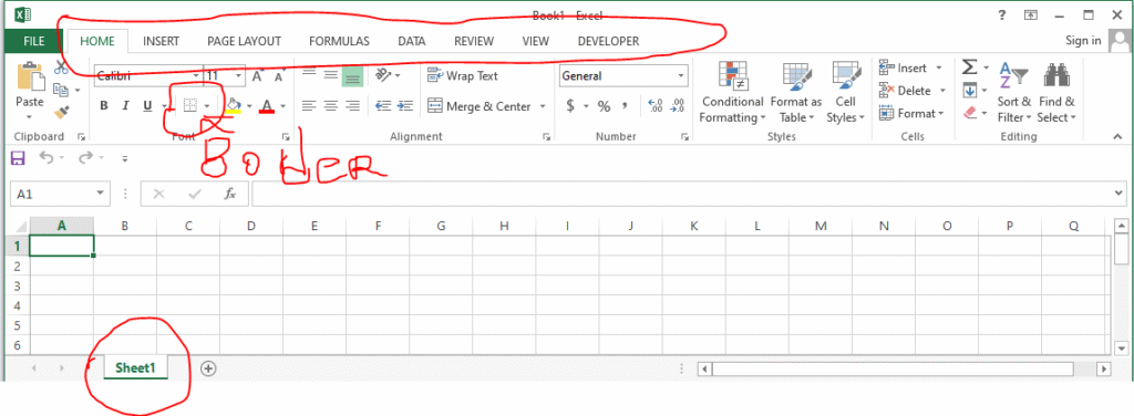
1. Opening Excel & Understanding the Interface

Open Excel → Select Blank Workbook.
Key Areas:
- Ribbon: Tabs like Home, Insert, Formulas with tools.
- Worksheet Grid: Rows (numbers) and columns (letters).
- Cell Address: The intersection of a row and column (e.g., A1, B2).

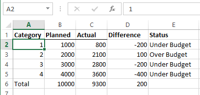
2. Entering Data

Example: Create a monthly budget.
- In cell A1, type: “Category”.
- In cell B1, type: “Planned”.
- In cell C1, type: “Actual”.
- Fill in categories (e.g., Rent, Groceries, Utilities) in A2 to A5.

3. Basic Formatting

Bold Headers: Select cells A1:C1 → Click B (Bold) in the Home tab.
Add Borders: Select the data range → Click the Border icon (🗎) → Choose a border style.
Adjust Column Width: Hover between column letters (e.g., A and B) → Drag to resize.

Part 2: Essential Formulas

1. Summing Values

In cell B6, type: =SUM(B2:B5) → Press Enter.
This adds all “Planned” expenses.
Repeat for C6 to sum “Actual” expenses.

2. Calculating Differences

In cell D1, type: “Difference”.
In cell D2, type: =C2-B2 → Press Enter.
Drag the fill handle (small square at the cell’s corner) down to D5 to copy the formula.

3. Using Functions

AVERAGE: In cell D6, type =AVERAGE(D2:D5) to see the average difference.
IF Statement:
In cell E1, type: “Status”.
In cell E2, type: =IF(D2<=0, "Under Budget", "Over Budget") → Drag down to E5.

Part 3: Creating a Chart

Select Data: Highlight A1:A5 and C1:C5 (hold Ctrl to select non-adjacent ranges).
Insert Chart: Go to the Insert tab → Choose a Clustered Column Chart.
Customize:

Click the chart title to rename it (e.g., “Actual vs. Planned Budget”).
Use the Chart Design tab to change colors or styles.

Part 4: Saving Your Work

Click File → Save As.
Choose a location (e.g., Desktop) and name your file (e.g., “My_Budget.xlsx”).
Select .xlsx as the file type → Click Save.

Practice Exercise

Create a “Sales Report” with:

Columns: Product, Q1 Sales, Q2 Sales, Total Sales.
Use SUM to calculate “Total Sales” for each product.
Add a bar chart comparing Q1 and Q2 sales.

Pro Tips

Keyboard Shortcuts:
Ctrl + C / Ctrl + V: Copy/Paste.
Ctrl + Z: Undo.
F2: Edit a cell.
AutoFill: Type “Jan” in a cell → Drag the fill handle to auto-generate “Feb”, “Mar”, etc.
Freeze Panes: Keep headers visible while scrolling (View → Freeze Panes).

Next Steps

Once comfortable with basics, explore:

Pivot Tables (summarize large datasets).
VLOOKUP/XLOOKUP (search for data in tables).
Conditional Formatting (highlight cells based on rules).